Introduction to Rigid Body Motion

In today’s post I want to explore the rigid body motion.

When a body moves, we can divide it into two distinct types of motion, a translation and a rotation. The translation can be treated with Newton’s Laws applied to the Center of Mass, but the rotation is a topic that often eludes people.

To try to develop the theory for the rotation of bodies we have to review the concept of a point mass particle, a body with negligible dimension, which means that rotation is undefined. How can we see if a point rotates? This means that rotation is a characteristic of sets of point particles and not of individual particles. This is the way we are going to define a rigid body of non-negligible dimensions, as a set of point particles whose distances between one another is constant.

Now that we know what we are studying, let’s define correctly the center of mass, a concept very important (and handy) for the study of rotations. The center mass corresponds to the position of the body (interior to the body or not) such that if the intire mass was compressed into that point, its motion could be accounted by only our knowledge so far of Newton’s equation. Imagine you throw a stick in the air with some rotation, there will be a point in the which will describe a parabola as predicted by the equations of a throw. The remaining points can be thought of translating with the center of mass (CM) and rotating around it.

The position of the center of mass can be calculated by:

$\vec R_{CM} = \sum_i \frac{\vec r_i m_i}{M_{total}}$

i corresponds to a point particle of the body and we are summing over all of them.

As I said before the motion of each particle can be understood as a translation with the CM as well as a rotation around it. This means that the displacement in a particle i is given by:

$d\vec r_i = d\vec R_{CM} + d\vec\phi \times \vec r'_i$

Where $d\vec\phi$ is the change in angle of the particle with respect to the CM and $r'_i$ is the position of the particle in relation to the CM. One thing we must point out is that since the body is rigid, the same rotation will affect all particles. Only this way is the distance between them preserved.

Now let’s try to find more about rotations by writing the energy of the system, which will be the sum of the kinetic energies of all particles ( $\frac{d\vec\phi}{dt} = \Omega \text{ , } \frac{d\vec R_{CM}}{dt} = V_{CM}$ )

$\sum_i \frac{1}{2}m_i (v_i)^2 = \sum_i \frac{1}{2}m_i (\vec V_{CM} + \vec \Omega\times \vec r'_i)^2$
$\sum_i \frac{1}{2}m_i ((V_{CM})^2 + 2\vec V_{CM}\cdot \vec \Omega\times \vec r'_i + (\vec \Omega\times \vec r'_i)^2) = \frac{M_{total}}{2}V_{CM}^2 + \sum_i m_i \vec r'_i \cdot \vec V_{CM}\times \vec \Omega + \sum_i \frac{1}{2}m_i(\vec \Omega\times \vec r'_i)^2)$

However since $r'_i$ are the distances in respect to the CM the weighted sum of all $m_ir'_i$ will be zero, hence our expression becomes:

$E_k = \frac{1}{2}M_{total}V_{CM}^2 + \sum_i \frac{1}{2}m_i(\vec \Omega\times \vec r'_i)^2)$

The energy then reinforces the idea that the motion is a translation of the CM plus a rotation around the CM.

Now let’s see if by expanding the energy of rotation we can find fundamental structure.

$E_{rot} = \frac{1}{2}\sum_i m_i (\vec \Omega \times \vec r'_i)^2$
$\vec\Omega\times\vec r'_i = (\Omega_y r'_{iz} - \Omega_z r'_{iy}) \hat x + (\Omega_z r'_{ix} - \Omega_x r'_{iz})\hat y + (\Omega_x r'_{iy} - \Omega_y r'_{ix})\hat z$
$E_{rot} = \frac{1}{2}\sum_i m_i ((\Omega_y r'_{iz} - \Omega_z r'_{iy})^2 + ( \Omega_z r'_{ix} - \Omega_x r'_{iz})^2 + ( \Omega_x r'_{iy} - \Omega_y r'_{ix})^2)$
$= \frac{1}{2}\sum_i m_i (\sum_k \Omega_k^2 (\sum_l r'^2_{il}) - \sum_{k,l} \Omega_k\Omega_l r'_{ik}r'_{il})$

This last summation part needs care, if you don’t see it at first, please read it carefully. Dropping the summation sign to make the notation less cumbersome we have:

$E_{rot}=\frac{1}{2}\sum_i m_i ( \Omega_k \Omega_l r'^2_{im} \delta_{kl} - \sum_{k,l} \Omega_k \Omega_l r'_{ik} r'_{il})$
$=\frac{1}{2}\Omega_k \Omega_l \sum_i m_i(r'^2_{im} \delta_{kl} - r'_{ik}r'_{il})$

We know define a new quantity, the tensor of inertia $I_{lk}$ where

$I_{lk} = \sum_i m_i(r'^2_{im} \delta_{kl}-r'_{ik}r'_{il})$

Then the rotation energy can be written simply as:

$T_{rot}=\frac{1}{2}\Omega_i\Omega_l I_{ik}$

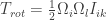
And $I$ written explicitely will be:

$I = \begin{bmatrix} \sum m(y^2 + z^2) & -\sum m(xy) & -\sum m(xz)\\ -\sum m(yx) & \sum m(x^2 + z^2) & -\sum m(yz) \\ -\sum m(zx) & -\sum m(zy) & \sum(m(x^2 + y^2) \end{bmatrix}$

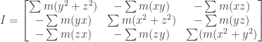
If the body is continuous we just transform the summations into integrals over the entire volume of the body.

So now the inertial moment of a body is not only a scalar, it actually depends on the various directions of the rotation.

However the is a cool result which states that it is always possible to find a set of directions such that $I$ is diagonal, which eases the mathematics of the problems as well as give us a better insight into the symmetries of the body. These directions are called the principal axis of the body.

The next point in our analysis will be developing an analog to the linear momentum for rotations, and then develop a analog to the Newton’s second equation but for rotations.

In the generalization of the momentum, we start by defining it as $m\vec r\times \vec v$ for a point particle. Then for a full body:

$\vec L = \sum_i m_i \vec r_i \times(\vec \Omega \times \vec r_i) = \sum m_i(r^2\vec \Omega - \vec r(\vec r\cdot \vec \Omega))$
$= \sum_i m_i(r_l^2\Omega_k - r_kr_l\Omega_l) = \Omega_l \sum_i m_i(r_l^2\delta_{kl} - r_kr_l) =\Omega_l I_{lk} = I \vec \Omega$

Deriving $\vec L$ :

$\frac{d}{dt}\vec L = \sum_i m_i( \dot{\vec r_i}\times \vec v_i + r_i \times \dot{\vec v_i}) = \sum_i m_i( \vec v_i \times \vec v_i + r_i \times \vec a_i)$
$= \sum_i r_i \times (m_i \vec a_i) = \sum_i r_i \times F_i = \vec \tau$

Now we found a quatity that varies our Angular momentum the same way as in Newton’s second law.

We now have the basis for the rigid body motion.

References: Landau Volume 1 Mechanics

Calculating derivatives of products using Pascal’s Triangle

The method

Suppose you wish to calculate the n-th derivative of the product of two functions $f$ and $g$ . There is a general rule, called Leibniz’s rule, which gives a slightly easier way of computing it, without the process of calculating every step. The rule states that

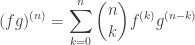$\displaystyle (fg)^{(n)}=\sum_{k=0}^n\dbinom{n}{k}f^{(k)}g^{(n-k)}$ .

So the n-th derivative is the sum of n+1 terms, with the coefficients given by the n-th line of Pascal’s triangle. This is very much like the binomial theorem, which states that, given two numbers $a$ and $b$ ,

$\displaystyle \left(a+b\right)^n=\sum_{k=0}^n\dbinom{n}{k}a^{k}b^{n-k}$ .

An example

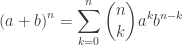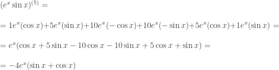
Suppose we wish to calculate $\left(e^x \sin x\right)^{(5)}$ . We will still need to calculate the first 5 derivatives of both functions, but that is pretty straight forward. We also calculate the 5th line of Pascal’s triangle.

$n$	$(e^x)^{(n)}$	$(\sin x)^{(n)}$
$1$	$e^x$	$\cos x$
$2$	$e^x$	$-\sin x$
$3$	$e^x$	$-\cos x$
$4$	$e^x$	$\sin x$
$5$	$e^x$	$\cos x$

					1
				1		1
			1		2		1
		1		3		3		1
	1		4		6		4		1
1		5		10		10		5		1

So, our derivative is simply multiplying the n-th coefficient with the n-th derivative of $e^x$ and the n-th derivate of $\sin x$ , but counting this last one backwards, starting from the bottom of the table.

$(e^x\sin x)^{(5)}= \\ \\ =1e^x(\cos x)+5e^x(\sin x)+10e^x(-\cos x)+10e^x(-\sin x)+5e^x(\cos x)+1e^x(\sin x)= \\ =e^x(\cos x+5\sin x-10\cos x-10\sin x+5\cos x+\sin x)= \\ \\ =-4e^x(\sin x +\cos x)$ .

Why does it work?

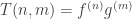
The idea behind both “rules” is that we apply an operation to a general term, which we shall call the term $T(n,m)$ . The operation $F$ is such that:

$F(~T(n,m)~)=T(n+1,m)+T(n,m+1)$

In particular, we have:
1) In the binomial theorem,
$T(n,m)=a^nb^m$ and F is multiplying by $(a+b)$ :
$F(~T(n,m)~)=a^nb^m(a+b)=a^{n+1}b^m+a^nb^{m+1}=T(n+1,m)+T(n,m+1)$

2) In Leibnitz’s rule,
$T(n,m)=f^{(n)}g^{(m)}$ and F is the derivative operator:
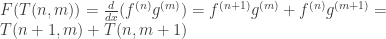
$F( T(n,m) )=\frac{d}{dx}(f^{(n)}g^{(m)})=f^{(n+1)}g^{(m)}+f^{(n)}g^{(m+1)}=\\ T(n+1,m)+T(n,m+1)$

Here, $+$ stands for standard addition. We must also state the initial condition,
$(a+b)^0=1\\ (fg)^{0}=fg$

So, we have the following theorem.
1) If $V$ is a vector space and $T(n,m)\in V$ for every non-negative m,n;
2) If there is an operation $F$ such that $F(~T(n,m)~)=T(n+1,m)+T(n,m+1)$ ,
then:
$\displaystyle F^n(T(0,0))=\sum_{k=0}^{n}\dbinom{n}{k}T(k,n-k)$ .

This generalizes both rules.

The idea of the proof was found here: http://math.stackexchange.com/questions/135510/how-is-leibnizs-rule-for-the-derivative-of-a-product-related-to-the-binomial-fo .

Two Timed approximation

The last post concerned about perturbation theory. A method used to approximate solution which was based on the idea of a solution we already know which has been slightly perturbed. Unfortunately this method is not always the best. Today I will present a different method called Two Timin in Strogatz’s “Nonlinear Dynamics and Chaos”

The idea of this approximation method is to make use of the different timescales of the function. To explain this idea I will use the example I will be solving afterwards.

Imagine you have damped harmonic oscillator. At first there doesn’t seem to exist two timescales, it is simply a harmonic motion whose amplitude decreases with time, however there are two time scales associated with the motion, the first gives us the timescale of the vibrations while the other gives the timescale of the exponential decrease. (more…)

Introduction to perturbation theory

In this post I will go through an introduction to perturbation theory, a method used to solve approximately differential equations that may not have solution otherwise. I will first go through the idea and then use an example, the non-linear oscillator to better explain the method.

The main idea of perturbation theory is to understand our system as a function/solution we know but which has been slightly perturbed. Imagine the case of ball rolling through a downhill straight valley. If the system was “at its best”, it would just go straight through the valley. However, if at the beginning we give it a little push to the side, it will go down, but also oscillate. We can think of the motion as the straight motion plus a small perturbation of the system.

(more…)

Integration Methods (Part 4)

Yesterday I covered a different integration methods, Heun’s method and we covered the reason why Euler’s method was not very accurate.

Today I will cover another integration method Runge-Kutta, which improves on the Heun’s method. Moreover I will touch on the subject of justifying why one method is better than another.

The basic idea of the Runge-Kutta method is to improve on the Heun’s method.
The improve this method (Heun’s) brought was to take into account the derivative not only at our current point, but also at, approximately, the end point, and from there get a better estimate of the average derivative in the interval.

Using the derivative at our first test point increases the accuracy of the step since, despite not being the derivative at our desired point, it will be a good approximation to it. So by averaging it with the the derivative at our start point we get a better approximation of the average value since we’ll take into some consideration the increase or decrease of the derivative in the time step.

As we saw this simple idea brought a great improvement on our method, however we can think how we can try to squeeze more information out of our system. Runge-Kutta method does just that.

(more…)

Integration Methods (Part 3)

Today’s article is about other numerical methods and why we need them.

Before discussing other numerical methods I will first show the pitfalls of the Euler method with a few examples. Then I will show two other numerical integration methods, which act on improving the Euler’s method, the improved Euler method and the Runga-Kutta method.

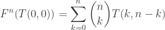First I will show the effect of the step size on the Euler’s Method. In the following picture we have the Euler’s mehtod solving the function $\dot x = x$ which gives rise to the exponential function.

Euler’s Method set size comparison

As we can see and intuitively know, by reducing the step size the method makes our method approach the exact solution, which in this graph is covered by the approximation with 0.001 step size.

Despite not having a comparison term, the time step required to get the precision we get here is too small, meaning that we need to make too many calculations and the code will run slowly.

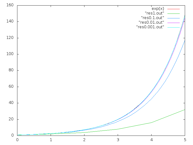
So why does the Euler’s Method has a error? We are using the derivative of the function at a point $\bf x$ to calculate the next step, to a point $\bf x + \delta x$ why is there an error?

The problem is that it is a finite step, while the real calculation of the integral the steps are infinitesimal. So by only making the step with the derivatives at the point $\bf x$ we are disregarding the motion of the derivative in the interval between $\bf x$ and $\bf x + \delta x$ . This is the source of the error in this method.

The next method tries to overcome that by taking a preemptive step and using the derivatives at the original point $\bf x$ and at the point $\bf x'$ to calculate $\bf x + \delta x$ . This method is called improved Euler’s formula or Heun’s method.

The algorithm is the following:

x = initial state
while t <TMAX:
    k1 = f(x) * DT
    k2 = f(x+k1)*DT
    x(t+DT) = x(t) + 0.5*(k1+k2)
    t = t+DT

f(x) is the vector function that returns a vector with the derivatives of $\bf x$ .

Like I said before the idea of the method is to take one first step and then use this step to calculate a the derivative of $\bf x$ .at that point. Since we are taking the derivatives of at approximately both ends of the step, the method will give out a better value for the average derivative in the interval when compared to the Euler Method. wiki

(This idea is also used in numerical integration and is more know as the trapezoid rule, wiki)

Plotting the same differential equation with this method yields.

Right away, we can see that the solution closes in the exact solution much faster, even though we have approximately double de calculations, we achieved the same precision with a step size of 0.1 with Heun’s method as almost 0.001 in Euler’s method. The same computation with 50x less calculations!

This is the power of a good numerical method. By using a better method we were able to better use our resources and still get the same result. If we were tackling a big problem requiring a big server that took , for example, 50 days of computation, by using this method we could reduce this time to 1 day! Allowing the other 49 days to be used for other tasks!

Note: the number of 50 is not a definite relationship between the efficiency of the two methods, it was just a value used for demonstration purposes. The correct factor will depend on the exact differential equation and implementation.

Tomorrow I will introduce a new integration method. See you then!

(The code used for the integration is available on github)

Integration Methods (Part 2)

Yesterday I went over the reason why we want to study numerical integration methods and introduced Euler’s method to give an idea on how integration methods work.In this post I will cover how to generalize the Euler’s method to many variables.

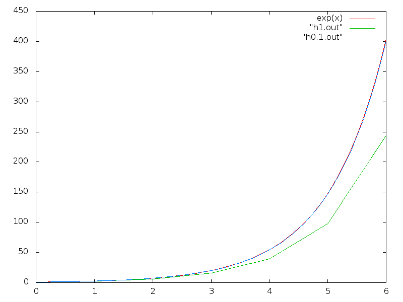
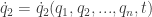
Imagine our system does not depend on one variable only, but instead depends on an arbitrary number of variables $q_1, q_2,..., q_n$ and maybe time such that we have their derivatives as a function of these variables:

$\dot q_1 = \dot q_1( q_1, q_2, ..., q_n, t)$

$\dot q_2 = \dot q_2( q_1, q_2, ..., q_n, t)$

…

$\dot q_n = \dot q_n( q_1, q_2, ..., q_n, t)$

(more…)

Integration Methods (Part 1)

I would like to have my first post with a topic I find very interesting, integration methods.Since the advent of computers they have been put to use to solve scientific problems. One of the biggest uses is to do numerical computations, either massive calculations or using computers to approximate solutions. This second comes as very important, specially in differential equations when we are faced with systems which do not have an analytic solution or closed formula, like:

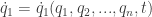
$\ddot \theta + k\sin(\theta) = 0$ – The system of a simple pendulum

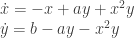$\begin{array} {l} \dot x = -x + ay + x^2y\\ \dot y = b -ay - x^2y \end{array}$ – Biological processes like glycolisis
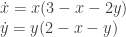$\begin{array} {l} \dot x = x(3-x-2y)\\ \dot y = y(2-x-y) \end{array}$ – Growth models of species

The study of these systems (despite existing a lot of techniques to deal with them) depend on our ability to approximate the solution from the differential equations.

It is for this reason that integration methods are very important. We need methods which can give us a very approximate solution with the minimum effort.

You may ask “but if it is the computers that do the calculations, why do we need to minimize effort?” The answer is simple, computers aren’t invincible, they have limitations, and if we ask too much from them they will take a long time to give us an answer, and sometimes we do not have that time, whether is just a scientist that needs results to continue his work or a company that needs the information as soon as possible to know what course they need to follow.

(more…)

42 Lactors

A little bit of knowledge everyday

Introduction to Rigid Body Motion

Calculating derivatives of products using Pascal’s Triangle

Two Timed approximation

Introduction to perturbation theory

Integration Methods (Part 4)

Integration Methods (Part 3)

Integration Methods (Part 2)

Integration Methods (Part 1)