The last post concerned about perturbation theory. A method used to approximate solution which was based on the idea of a solution we already know which has been slightly perturbed. Unfortunately this method is not always the best. Today I will present a different method called Two Timin in Strogatz’s “Nonlinear Dynamics and Chaos”
The idea of this approximation method is to make use of the different timescales of the function. To explain this idea I will use the example I will be solving afterwards.
Imagine you have damped harmonic oscillator. At first there doesn’t seem to exist two timescales, it is simply a harmonic motion whose amplitude decreases with time, however there are two time scales associated with the motion, the first gives us the timescale of the vibrations while the other gives the timescale of the exponential decrease.
The idea becomes to write our function of time, as a function of two times 


Then if we have:

We can also write:

Now like perturbation theory we take our function to be power series on the same variable


Now let’s use an example to better understand this method. We are going to try to solve the damped harmonic oscillator, a system we know the solution however will serve fine to illustrate the method. 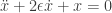
Let’s write with our approximation. (We just want an approximation to the first order of


![\partial_{\tau\tau}x_0 + x_0 + \epsilon[ 2\partial_\tau x_0 +2\partial_{\tau T} x_0 + \partial_{\tau\tau}x_1 + x_1] + O(\epsilon^2) = 0](https://s0.wp.com/latex.php?latex=%5Cpartial_%7B%5Ctau%5Ctau%7Dx_0+%2B+x_0+%2B+%5Cepsilon%5B+2%5Cpartial_%5Ctau+x_0+%2B2%5Cpartial_%7B%5Ctau+T%7D+x_0+%2B+%5Cpartial_%7B%5Ctau%5Ctau%7Dx_1+%2B+x_1%5D+%2B+O%28%5Cepsilon%5E2%29+%3D+0+&bg=ffffff&fg=333333&s=0&c=20201002)
Since we have two set of terms of different order of magnitude we can say that both must equal 0, meaning:


Since the partial derivatives in the first equation are in respect to 

Plugging in 

(Remember that we take funtions of 
However the equation we have gives rise to ressonance, which cannot be true, since it would imply that 


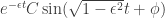
This means we have our solution for

Even not considering the other terms we it to be very close to the actual solution.
Although this case is not very representative, the method outline here can be used to approximate a function which has different timescales. It also becomes a good way of predicting to what values a system evolves and stabilizes on.


References: “Nonlinear Dynamiscs and Chaos” – Steven H. Strogatz
