In this post I will go through an introduction to perturbation theory, a method used to solve approximately differential equations that may not have solution otherwise. I will first go through the idea and then use an example, the non-linear oscillator to better explain the method.
The main idea of perturbation theory is to understand our system as a function/solution we know but which has been slightly perturbed. Imagine the case of ball rolling through a downhill straight valley. If the system was “at its best”, it would just go straight through the valley. However, if at the beginning we give it a little push to the side, it will go down, but also oscillate. We can think of the motion as the straight motion plus a small perturbation of the system.
The idea becomes then to describe the motion 


With this introduction let’s move on to the example of a non-linear oscillator.
Imagine we have an oscillator which does not have a force proportional to the displacement, but the force is also dictated by higher order terms of displacement.
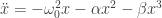
This is a non-linear differential equation which we don’t know how to solve. However we see an important aspect, if the motion does not have a great amplitude, then we have that the terms of 

If with take into account the idea of perturbations we know the solution will be a harmonic oscillator a bit perturbed and that is going to be our first step.
First let’s write 
The term of order zero of amplitude will be 
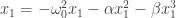
Now we take the first order approximation, in this case we take 
Since 


(We are disregarding phase since it does not alter the problem and would only make the notation more cumbersome.)
Note an important thing, I wrote on the solution of 

Then we need to write:

We know
Now to find the second term, we need to find the solution of the equation to the second order of amplitude. We then include 

Substituting 
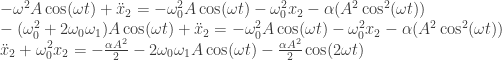
Now we stop and look at our equation. It now is solvable, it is the equation of a driven harmonic oscillator. However look at the driving frequency of the middle term, it is 

Notice also that we neglected any terms of order greater than 2, both on 
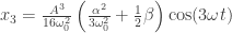
The solution then becomes:

Notice that as we wanted, 

![\ddot x_3 + \omega_0^2 x_3 = A^3 \left[ -\frac{1}{4} \beta - \frac{\alpha^2}{6\omega_0^2} \right] \cos(3\omega t) + A\left[ 2\omega_0\omega_3 + \frac{5A^2\alpha^2}{6\omega_0^2} - \frac{3}{4}A^2\beta \right] \cos(\omega t)](https://s0.wp.com/latex.php?latex=%5Cddot+x_3+%2B+%5Comega_0%5E2+x_3+%3D+A%5E3+%5Cleft%5B+-%5Cfrac%7B1%7D%7B4%7D+%5Cbeta+-+%5Cfrac%7B%5Calpha%5E2%7D%7B6%5Comega_0%5E2%7D+%5Cright%5D+%5Ccos%283%5Comega+t%29+%2B+A%5Cleft%5B+2%5Comega_0%5Comega_3+%2B+%5Cfrac%7B5A%5E2%5Calpha%5E2%7D%7B6%5Comega_0%5E2%7D+-+%5Cfrac%7B3%7D%7B4%7DA%5E2%5Cbeta+%5Cright%5D+%5Ccos%28%5Comega+t%29&bg=ffffff&fg=333333&s=0&c=20201002)
(Left as an exercise to get there)
Since we need to remove any resonant terms we must set:

Giving us 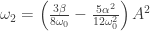
We can then solve for 
Note how the terms we found are of the order of amplitude we predicted them to be.
In conclusion, the perturbation theory is a good method to obtain approximations to the real solution of situation where we have a motion that was perturbed from a normal behavior. Its ability to approximate depends, however, on the size of the perturbation and the nature of the perturbation. When necessary to do an approximation using this method, check that the size of the amplitude still allows for the increase in order of smallness as you find more terms.
References: Laundau Volume 1 – Mechanics
