Mathematics

Calculating derivatives of products using Pascal’s Triangle

The method

Suppose you wish to calculate the n-th derivative of the product of two functions $f$ and $g$ . There is a general rule, called Leibniz’s rule, which gives a slightly easier way of computing it, without the process of calculating every step. The rule states that

$\displaystyle (fg)^{(n)}=\sum_{k=0}^n\dbinom{n}{k}f^{(k)}g^{(n-k)}$ .

So the n-th derivative is the sum of n+1 terms, with the coefficients given by the n-th line of Pascal’s triangle. This is very much like the binomial theorem, which states that, given two numbers $a$ and $b$ ,

$\displaystyle \left(a+b\right)^n=\sum_{k=0}^n\dbinom{n}{k}a^{k}b^{n-k}$ .

An example

Suppose we wish to calculate $\left(e^x \sin x\right)^{(5)}$ . We will still need to calculate the first 5 derivatives of both functions, but that is pretty straight forward. We also calculate the 5th line of Pascal’s triangle.

$n$	$(e^x)^{(n)}$	$(\sin x)^{(n)}$
$1$	$e^x$	$\cos x$
$2$	$e^x$	$-\sin x$
$3$	$e^x$	$-\cos x$
$4$	$e^x$	$\sin x$
$5$	$e^x$	$\cos x$

					1
				1		1
			1		2		1
		1		3		3		1
	1		4		6		4		1
1		5		10		10		5		1

So, our derivative is simply multiplying the n-th coefficient with the n-th derivative of $e^x$ and the n-th derivate of $\sin x$ , but counting this last one backwards, starting from the bottom of the table.

$(e^x\sin x)^{(5)}= \\ \\ =1e^x(\cos x)+5e^x(\sin x)+10e^x(-\cos x)+10e^x(-\sin x)+5e^x(\cos x)+1e^x(\sin x)= \\ =e^x(\cos x+5\sin x-10\cos x-10\sin x+5\cos x+\sin x)= \\ \\ =-4e^x(\sin x +\cos x)$ .

Why does it work?

The idea behind both “rules” is that we apply an operation to a general term, which we shall call the term $T(n,m)$ . The operation $F$ is such that:

$F(~T(n,m)~)=T(n+1,m)+T(n,m+1)$

In particular, we have:
1) In the binomial theorem,
$T(n,m)=a^nb^m$ and F is multiplying by $(a+b)$ :
$F(~T(n,m)~)=a^nb^m(a+b)=a^{n+1}b^m+a^nb^{m+1}=T(n+1,m)+T(n,m+1)$

2) In Leibnitz’s rule,
$T(n,m)=f^{(n)}g^{(m)}$ and F is the derivative operator:
$F( T(n,m) )=\frac{d}{dx}(f^{(n)}g^{(m)})=f^{(n+1)}g^{(m)}+f^{(n)}g^{(m+1)}=\\ T(n+1,m)+T(n,m+1)$

Here, $+$ stands for standard addition. We must also state the initial condition,
$(a+b)^0=1\\ (fg)^{0}=fg$

So, we have the following theorem.
1) If $V$ is a vector space and $T(n,m)\in V$ for every non-negative m,n;
2) If there is an operation $F$ such that $F(~T(n,m)~)=T(n+1,m)+T(n,m+1)$ ,
then:
$\displaystyle F^n(T(0,0))=\sum_{k=0}^{n}\dbinom{n}{k}T(k,n-k)$ .

This generalizes both rules.

The idea of the proof was found here: http://math.stackexchange.com/questions/135510/how-is-leibnizs-rule-for-the-derivative-of-a-product-related-to-the-binomial-fo .

Integration Methods (Part 3)

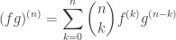
Today’s article is about other numerical methods and why we need them.

Before discussing other numerical methods I will first show the pitfalls of the Euler method with a few examples. Then I will show two other numerical integration methods, which act on improving the Euler’s method, the improved Euler method and the Runga-Kutta method.

First I will show the effect of the step size on the Euler’s Method. In the following picture we have the Euler’s mehtod solving the function $\dot x = x$ which gives rise to the exponential function.

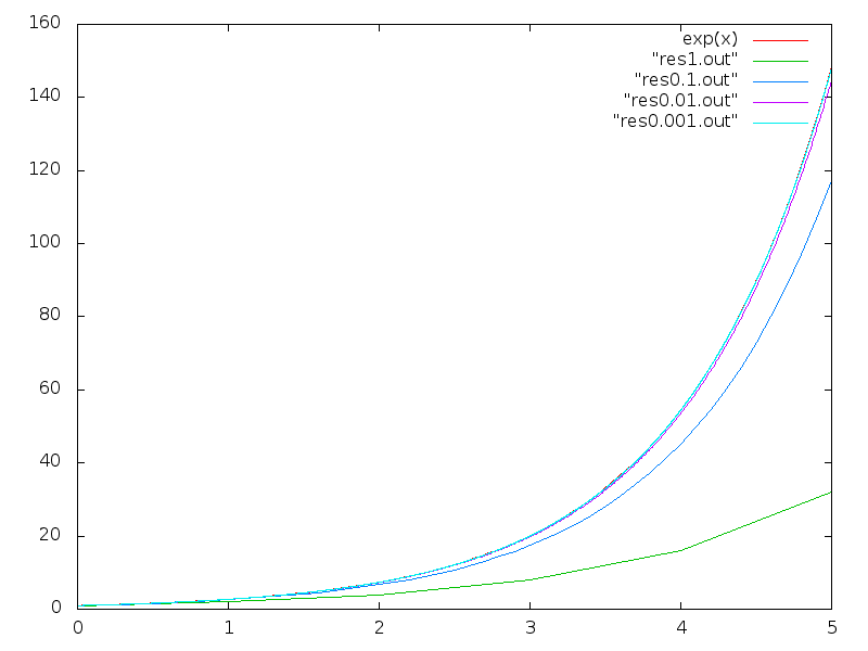
Euler’s Method set size comparison

As we can see and intuitively know, by reducing the step size the method makes our method approach the exact solution, which in this graph is covered by the approximation with 0.001 step size.

Despite not having a comparison term, the time step required to get the precision we get here is too small, meaning that we need to make too many calculations and the code will run slowly.

So why does the Euler’s Method has a error? We are using the derivative of the function at a point $\bf x$ to calculate the next step, to a point $\bf x + \delta x$ why is there an error?

The problem is that it is a finite step, while the real calculation of the integral the steps are infinitesimal. So by only making the step with the derivatives at the point $\bf x$ we are disregarding the motion of the derivative in the interval between $\bf x$ and $\bf x + \delta x$ . This is the source of the error in this method.

The next method tries to overcome that by taking a preemptive step and using the derivatives at the original point $\bf x$ and at the point $\bf x'$ to calculate $\bf x + \delta x$ . This method is called improved Euler’s formula or Heun’s method.

The algorithm is the following:

x = initial state
while t <TMAX:
    k1 = f(x) * DT
    k2 = f(x+k1)*DT
    x(t+DT) = x(t) + 0.5*(k1+k2)
    t = t+DT

f(x) is the vector function that returns a vector with the derivatives of $\bf x$ .

Like I said before the idea of the method is to take one first step and then use this step to calculate a the derivative of $\bf x$ .at that point. Since we are taking the derivatives of at approximately both ends of the step, the method will give out a better value for the average derivative in the interval when compared to the Euler Method. wiki

(This idea is also used in numerical integration and is more know as the trapezoid rule, wiki)

Plotting the same differential equation with this method yields.

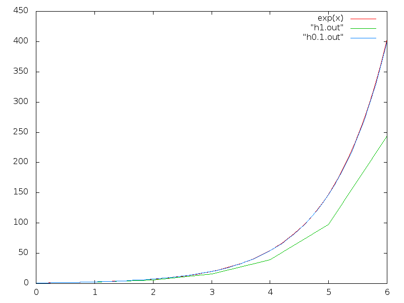
Right away, we can see that the solution closes in the exact solution much faster, even though we have approximately double de calculations, we achieved the same precision with a step size of 0.1 with Heun’s method as almost 0.001 in Euler’s method. The same computation with 50x less calculations!

This is the power of a good numerical method. By using a better method we were able to better use our resources and still get the same result. If we were tackling a big problem requiring a big server that took , for example, 50 days of computation, by using this method we could reduce this time to 1 day! Allowing the other 49 days to be used for other tasks!

Note: the number of 50 is not a definite relationship between the efficiency of the two methods, it was just a value used for demonstration purposes. The correct factor will depend on the exact differential equation and implementation.

Tomorrow I will introduce a new integration method. See you then!

(The code used for the integration is available on github)

Integration Methods (Part 2)

Yesterday I went over the reason why we want to study numerical integration methods and introduced Euler’s method to give an idea on how integration methods work.In this post I will cover how to generalize the Euler’s method to many variables.

Imagine our system does not depend on one variable only, but instead depends on an arbitrary number of variables $q_1, q_2,..., q_n$ and maybe time such that we have their derivatives as a function of these variables: