Yesterday I went over the reason why we want to study numerical integration methods and introduced Euler’s method to give an idea on how integration methods work.In this post I will cover how to generalize the Euler’s method to many variables.
Imagine our system does not depend on one variable only, but instead depends on an arbitrary number of variables 
…
The method then becomes a generalization of the Euler’s method in the following sense. We can think of the vector of the variables 
Then the value of the coordinates at a time 

The idea of introducing the coordinates as belonging in a vector structure was more than just to ease on the notation in this post. This idea lends to two important points:
- Representation:
By thinking of the states of the system as a vector and its derivative in a vector as well, it becomes easier to understand how we can represent a system and its derivatives.
Using a reference frame, we can plot the evolution of the system as the trajectory of the point 
Another way we can use the vector nature of our definitions is to define the vector field of the derivatives. In this picture we associate to each point (usually a lattice of points) with the vector of the derivative at that point. Since the trajectories are tangent to their derivatives we have that this vector field gives out the flow of the trajectories. This is good to get a good sense of the global behavior of the system, however it does not give you the rigor of a specific trajectory.
- Implementation
Linear algebra is very important in computer simulations and for that it is ,not only available in most (if not all) programming languages, but usually has a great performance, since its use is normally simulations. Writing our methods in terms of linear algebra terms will allow us two things, make use of optimized code as well as reduce the amount of code we have to write.
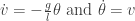
We know now how to do numerical integration on n variables, but what if our variables are themselves derivatives of other? For example, in the case of the pendulum where we have the second derivatives of the angle how can we do? Certainly our method must be different to accommodate this relationship between the variables

Well, in fact we can disregard that there is any second-derivative relationship between the two defining a new variable 
This is a system of differential equations like the one we saw above, and we can easily calculate the Euler’s method for this system.
To summarize, the idea is then to turn the higher derivatives of the initial variable into new variables of the system and then use the normal vector Euler’s Method.
Tomorrow I will cover other integration methods.
